Aggregates of carbon black with various shapes in a suspension were investigated to understand their behavior in fluid flow. At a lower aspect ratio, the particles exhibited tumbling or rotational motion, and the fluid flow was deflected in regions where the density of particles was higher. The contact between the particles promoted partial particle grouping when the aspect ratios of the particles were low. The average transitional motion of the particles was greatest at the lowest aspect ratio case. This led to weaker rearrangement event than those when the particles were nearly spherical. The elongated particles could act as bridges to promote the formation of particle groups. We believe that our study provides insight for suspensions containing particles with various shapes, which can be used to control the suspensions rheologically.

· Investigation of aggregation of carbon black with various shapes in a suspension. · Particles exhibited tumbling or rotational motion.

Keywords: non-Newtonian flow, aggregate, suspension, shear flow, lattice Boltzmann method

Suspensions containing nano-scale particles can be used in many industrial applications, such as solar energy harvesting,^1,2 lithium ion battery technology,³ and coating processes.⁴ In such applications, understanding colloidal particle dynamics in a suspension has been a major issue for reducing the harmful effects successfully, such as jamming, unequal surfaces, and broken devices.⁵ Furthermore, the final properties of micro- or nano-composites depend on the characteristics of the particle arrangements or matrix caused by their interactions or shapes. These characteristics can provide fundamental knowledge for suspensions. As a representative application example of suspensions in the coating and printing fields, the high degree of pigment dispersion and concentration⁶ of carbon black are important for the final product quality.⁷ Thus, the concentration of the dispersed phase also strongly affects the performance, as does an optimized solution viscosity.⁸ Thus, a deep understanding of suspensions is required to maintain the quality. Recently, there have been many approaches to unveil the complicated suspension phenomena experimentally. Many researchers have investigated the structures of carbon black aggregates using various techniques, including scanning electron microscopy (SEM)^9,10 and the transmission electron microscopy (TEM).¹¹ When using these methods, it is necessary to overcome their disadvantages, such as the short observation times and complicated sample preparation, to obtain a relevant experimental data. Furthermore, measuring the quality of the dispersion or aggregates, which can affect the overall viscosity of the suspension, is not simple. Recently, a numerical study of the rheology was conducted, which has been valuable for the manufacture of topical products. The famous approaches of the modeling of the rheological behavior of suspensions is Stokesian dynamic (SD) that is well suited to describe the particle-fluid interaction.¹² Safdari et al. researched particles immersed in fluid using Lattice–Boltzmann method (LBM) and the 4th Runge-kutta method.¹³ Sun et al. developed an algorithm to solve particle transport processes by combined finite volume method (FVM) - discrete element method (DEM).¹⁴

In this study, to examine the characteristics of carbon black particle aggregates, we generated aggregate structures with various shapes. The shapes of the particle aggregates were mainly elongated and dendritic. The mechanism of aggregate formation was as follows. All the primary particles were initially in a state of random motion. Due to the collisions between particles, particle groups formed. These grouped particles moved randomly in the fluid. When two groups collided, they merged into one cluster. These merged clusters must be controlled to control the suspension characteristics for applications. Different dendritic aggregates can be distinguished by their characteristic fractal exponents, which depend on the cluster growth,¹⁵ and various spherical or ellipsoidal shapes may form.¹⁶ There have many numerical studies on the dynamics of perfectly spherical micro- or nano-particles in linear shear flow. However, the anisotropic orientation of non-spherical particles is not well understood. We used a combined Eulerian-Lagrangian simulation to examine aggregates of carbon particles in shear flow and discuss the dependence of the aggregate shape. Our interest was the effect of particle-particle and particle-fluid interactions, neglecting the effects of ballistic cluster-cluster aggregation, which is often observed in carbon black processing.^17-19

This paper is structured as follows. In Section 2, we introduce the numerical modelling method. In Section 3, the calculated results are shown, and conclusions are presented in Section 4.

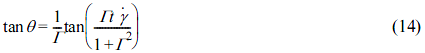
Modelling Aggregates. Figure 1 shows several asymmetric dendritic aggregates.^20,21 For simplicity, the center of mass and average area were computed, and the aggregates were approximated as ellipses with major and minor axes. This model also assumed that porosity of the carbon aggregates was 59% in which density is decreased with increasing amounts of interstitial fluid, if porosity is increased. Furthermore, in this study the carbon aggregates were non-fractal and had higher resistance to shear flow and stable structure, and the restructuring behaves depending on the connectivity of the primary particles was neglected.

Lattice–Boltzmann Method (LBM). While the LBM has been applied in fields ranging from image processing to quantum mechanics, it has historically been as a computational fluid dynamics method.²² It decomposes the continuous fluid into moving or resting pseudo-particles over a lattice domain. In this study, the D2Q9 model, which is the most popular model in 2-dimensional LBM calculations, was implemented. The density functions were calculated by the lattice Boltzmann equation (LBE) with the Bhatnagar–Gross–Krook (BGK) operator as follows:

where the left side represents the streaming part, the right side represents the collision part, f is the density distribution fuction, x is the space position, t is time, α is the velocity direction, and τ is the dimensionless relaxation time (in this study, τ = 1.0). The force density F_i is particularly important for coupling the fluid and the surface of a particle.

In eq. (1), the equilibrium distribution function f^eq is definded as follows:

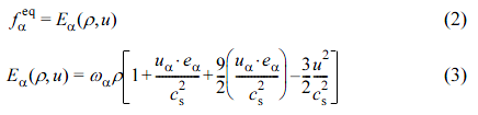
The weighting factor for the D2Q9 model is 4/9 for α = 0; 1/9 for α = 1, 2, 3, 4; and 1/36 for α = 5, 6, 7, 8. Figure 2 illustrates the momentum discretization for a two-dimensional calculation, where the virtual fluid particles at each node move to eight intermediate neighbors with eight corresponding velocity vectors:

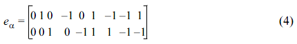
The macroscopic values are defined by the following equations:

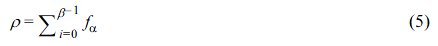
where β is 9 in the D2Q9 model.

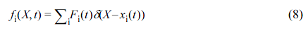
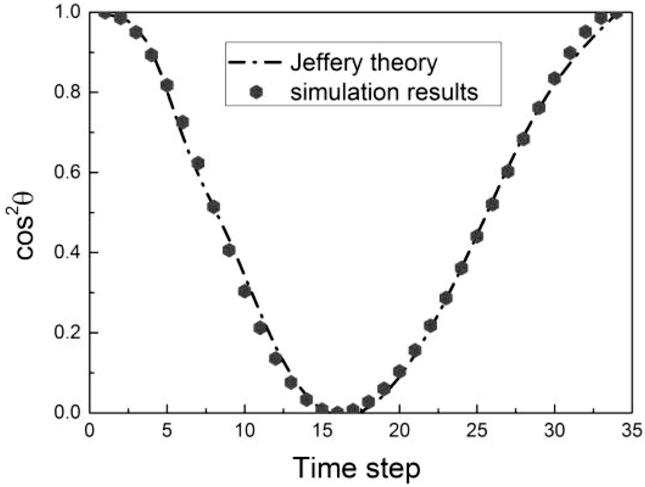
Immersed Boundary Method. The immersed boundary method (IBM) developed by Peskin²³ is used to simulate membranes containing particle nodes i in fluid flow and to couple the Eulerian coordinate system of a fluid lattice and the Lagrangian coordinates of particle surfaces, as shown in Figure 2. Each point of the particle surface is affected by the interactions between the incompressible viscous fluid force f_i(t) on the fluid nodes at time step t. The particle nodes i located at x_i(t) and X are fixed positions on the fluid lattice node. The Lagrangian force of each node F_i(t) is defined as follows:

where k is the stiffness parameter (input k = 0.3 for non-deformable surfaces), and x_i^ref(t) is the fixed reference position. Each point x_i(t) can translate from the reference position.

The Eulerian body force density f_i(X,t) was calculated from the Lagrangian force f_i(t) as follows:

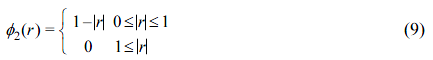
where the kernel δ(X - x_i(t)) is a discretized Dirac delta function with a finite support. Under the action of the distributed fluid forces, the particles’ motion is determined by their displacements and velocities. In this study, the interpolation function (φ_n, n= 2) was selected for the common decomposition, δ(r) = φ(x)φ(y):

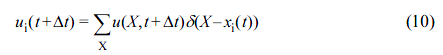
The new velocity u_i(t + 1) of the particle surface nodes i were calculated by the interpolation step as follows:

Furthermore, the no-slip condition was imposed at the surfaces of the particles. Finally, each particle surface node i could be moved explicitly by the Euler rule:

Discrete Element Method. A widely used approach for modeling a solid phase is the discrete element method (DEM), originally derived from molecular dynamics by Cundall et al.,²⁴ where the explicit temporal integration of the momentum balance is calculated. In this study, each node i on the particle surface were treated as discrete elements. The calculation of the Van der Waals Fi^→VDW  acting on each particle node i was included as follows:

Dispersed particles immersed in a fluid are affected Van der Waals forces if the suspension is colloidal.²⁵ Thus, the effect of Van der Waals forces was crucial in this work,²⁶ and the forces were calculated as follows:

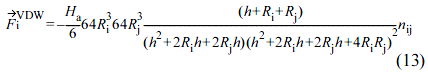
where R is the radius of particle, H_a is the Hamaker constant, which depends on the material (in this study, H_a = 8e^-20J), h(h = R_ij - R_i - R_j) is the distance between particles, and n_ij is the unit vector. To avoid the Van der Waals force paradox,²⁷ Fi^→VDW was set to zero when the value between nodes was 1 nm. Furthermore, when a particle contacted other particles, the force became repulsive, and the opposite direction of the force was used. Only the Van der Waals forces were considered (electrostatic interactions were ignored), because the Van der Waals forces should be dominant in systems with colloidal carbon black units, and electrostatic interactions are strongly screened.^28,29

Lattice–Boltzmann Immersed Boundary Discrete Element Method (LBIBDEM) Scheme. Each time step of the LBIBDEM scheme consisted of the following:

(1) At the first time step t, the node on the particles x_i(t) and the fluid state (u(X,t), ρ(X,t)) were known.

(2) The force density F(X,t) at the nodes was calculated from the surface stress using eq. (13) after unit rescaling.

(3) The boundary node force F(X,t) was spread to the Eulerian grid via IBM.

(4) f_i(X,t) was used in the LBM to compute the new state of the fluid u(X,t + 1), ρ(X,t)

(5) The new velocity u_i(t + 1) of the surface nodes were computed in the framework of the IBM using eq. (10)

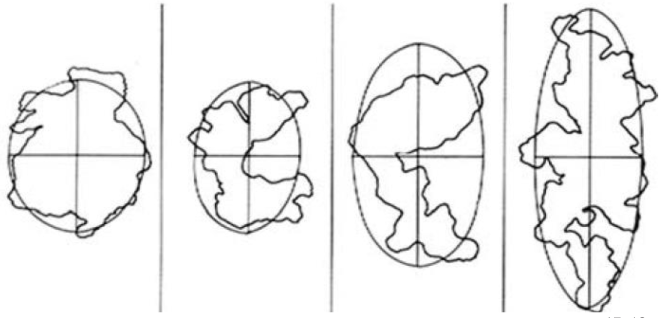
Validation. To validate our model, the Jeffery’s orbit of a suspended spheroid in an unbounded shear flow was used.³⁰ The theoretical solution by Jeffery for the rotational motion of the main symmetry axis was as follows:

where Γ = c/a, and a is the particle semi-axis with the highest degree of symmetry. The particle was positioned initially on the center of the fluid domain. Figure 4 shows the good agreement between the simulation and theoretical results. Figure 3

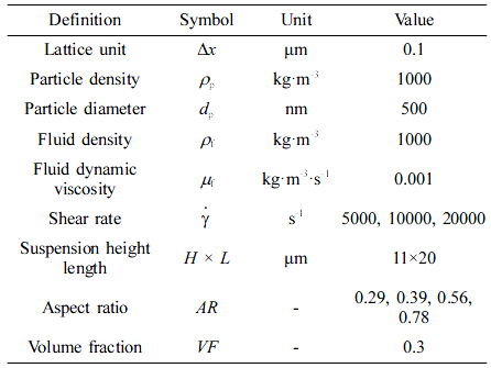
Simulations were carried out over a 110×200 lattice grid (11 μm×20 μm per lattice unit: Δx = 0.1 μm) with particles (diameter d_p = 500 nm). We assumed that the inside particles and the ambient fluid had identical properties (ρ_p = ρ_f). The detailed simulation parameters are listed in Table 1.

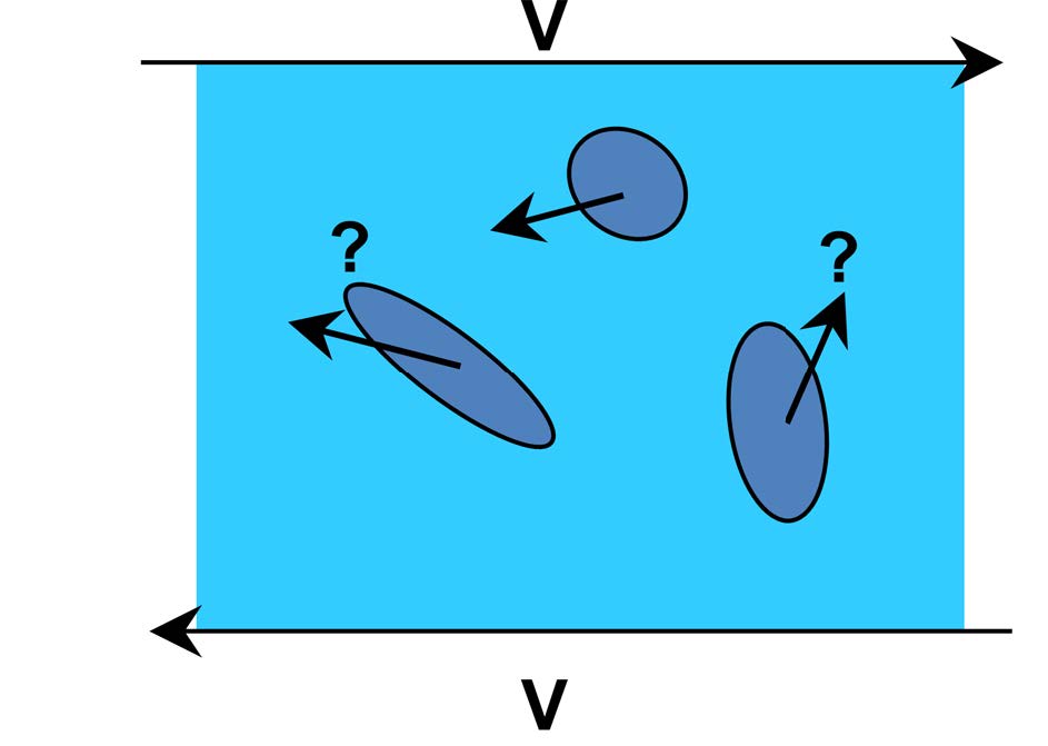
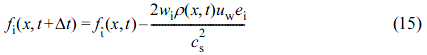
The halfway bounce-back³¹ scheme was applied on the upper and lower walls as follows:

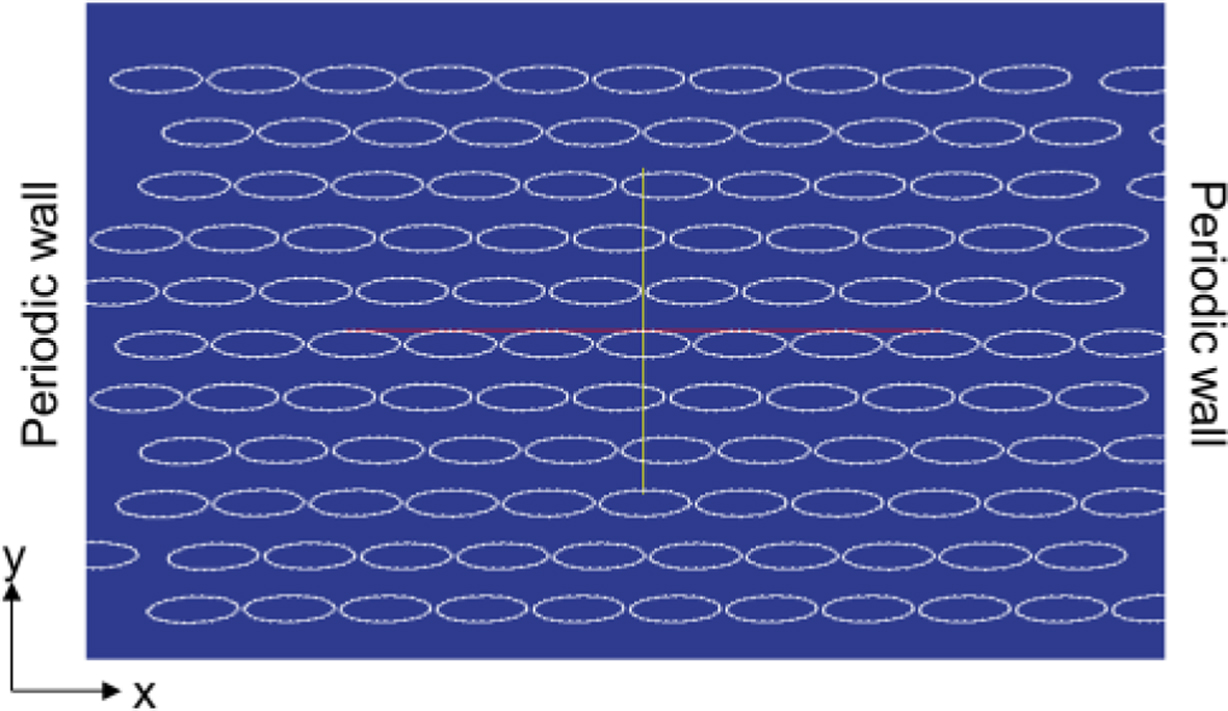
where is the fluid distribution after collision and  is the inverse direction of i and u_w is the velocity along the wall. Periodic boundary conditions were applied on the right, a and u_w is the velocity along the wall. Periodic boundary conditions were applied on the right, and left walls,³² as shown in Figure 5. Four different aggregate shapes were considered by changing the aspect ratio AR, as summarized in Table 1, and the total area of the particles in all the cases was maintained. The algorithm for successfully determining the particle behavior must be chosen based on the following considerations. If the mesh on the particle surface is too coarse, there may be ‘holes’ in the particle surface and fluid may penetrate. If the mesh is too fine, velocity interpolations become less accurate, which can cause the simulation to crash. Due to the finite-range interpolations, the flow field around the particle surface would be about 0.3–0.5 Δx(the lattice spacing).³³ The selected value in this study for the distance between nodes was 0.5 Δx. The initial configuration of the particles in the fluid domain is shown in Figure 6. In this study, the Brownian motion was neglected due to the high Peclet number. The Stokes number St for this system was about 0.0013, which indicates that fluid-solid coupling was strong and could lead to non-Newtonian behavior when St ≪1.³⁴

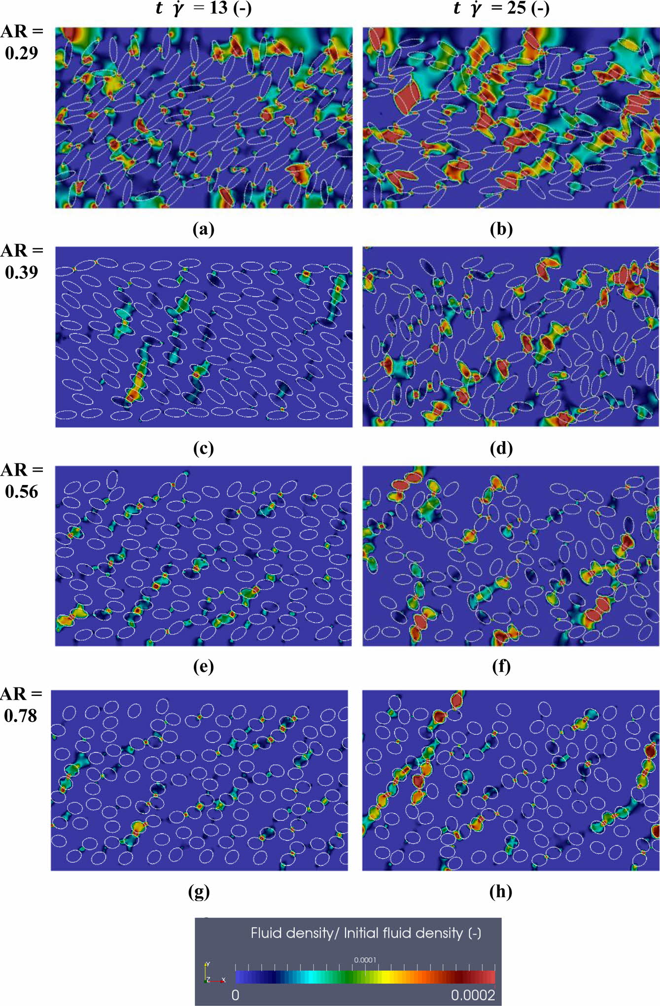
As shown in Figure 7, as AR varied, fluid density distributions in the calculated fluid domain appeared for AR = 0.29–0.78 at non-dimensional times of 13 and 25, separately. At a non-dimensional time of 13, the particles tended to move along the flow direction for all cases. The particles near the wall with an applied shear force nearly maintained their initial state, except when AR = 0.29. However, the particles located near the centerline experienced tumbling motion with an ordered structure. At a non-dimensional time of 25, the particles exhibited disordered structures for all cases. The spheroidal particles showed intriguing behaviors, especially for AR =0.29 and 0.39, as shown in Figures 7(a)-(d), in which their shapes promoted rolling or tumbling motions when a shear flow was applied.²⁵ Such remarkable particle behaviors led to more connections with the surrounding particles with steric interactions, binding the particle hydrodynamic cluster chains. The rotational motion determined the motion characteristics of almost all the particles at high particle Reynolds numbers.³⁵ Based on the interactions between the tumbling and rotational motions from the vorticity caused by the shear flow and the collisions with obstacles by the translational motion of the particles, the repulsion on the particle surfaces were due to hydrodynamic effects. Furthermore, in the higher density regime, i.e., over-crawling regime, the distribution expanded partially with decreasing AR, where particles tend to push into groups.³⁶ The elongated surfaces of the particles led to partial concentrations for two reasons: the deflection of the flow lines of the fluid surrounding the particles was less sensitive for the same-sized spheres, and the increased particle surface enhanced the probability of particle-particle interactions. This frequently occurs for high shear rates and high particle volume fractions because the microstructure transitions to a disordered state.³⁷ Above AR = 0.56, the particles with flowing fluid exhibited uniform alignment because the number of particle-particle interactions decreased, and these particles could change their orientation to the flow direction (x-direction). For the highest value of AR examined, which was close to a spherical shape (AR = 0.78), the simpler geometry and lower surface area than those of the oblate spheroidal aggregate experienced a reduction in friction, which promoted a sliding process.

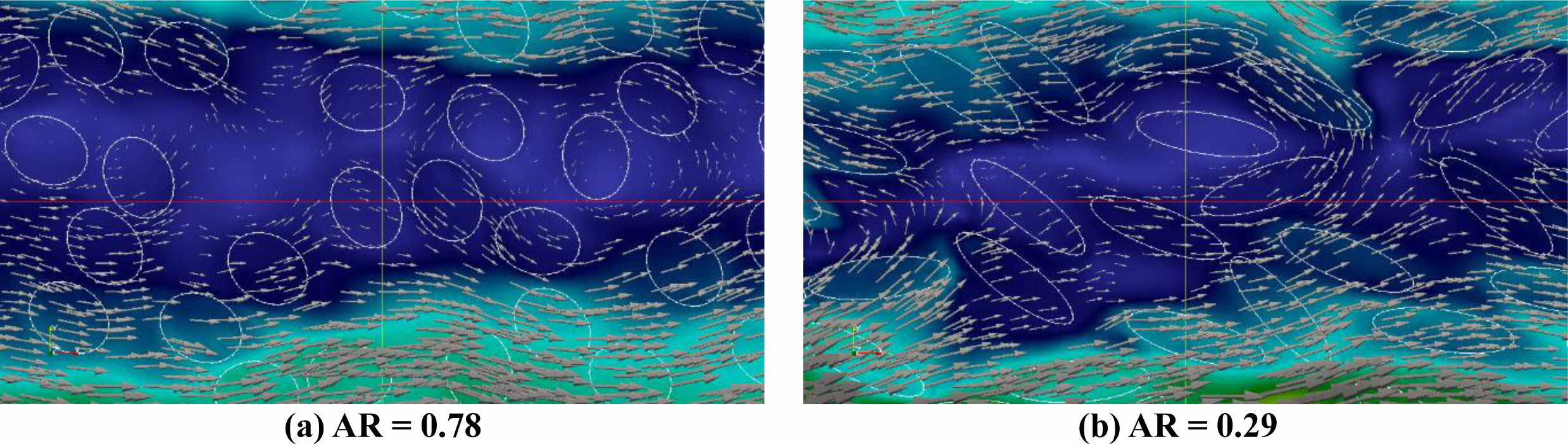
To better understand the relationship between the particles and fluid, the fluid velocity magnitude contours and vector field near the center region are shown in Figures 8(a) and 8(b), respectively. The vector size in this figure corresponds to the velocity magnitude. The deflection of flow lines by vectors near the particles for AR = 0.29 was stronger than that in the case of AR = 0.78. Thus, the particle positions can alter the fluid patterns, resulting in regions of high particle concentrations.

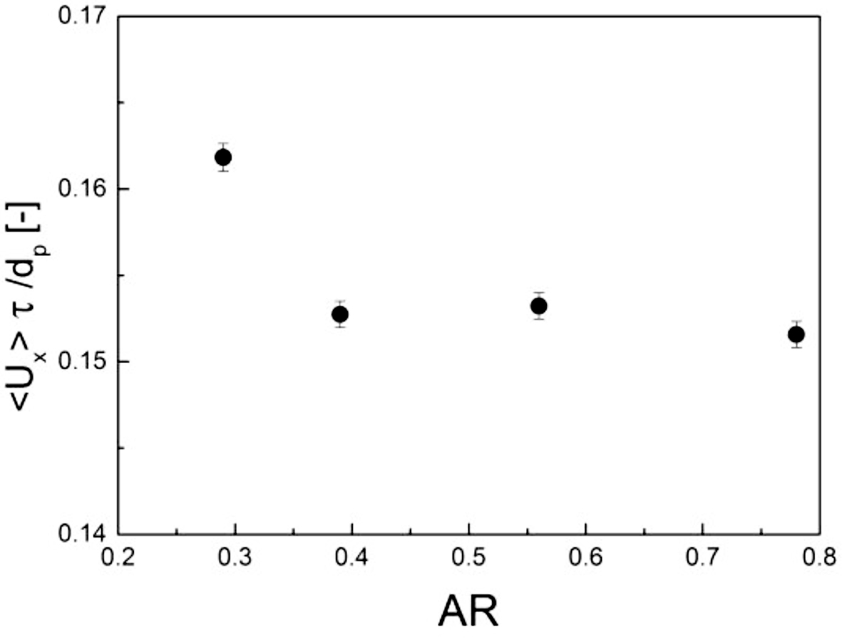
The translational velocity v_x along the shear flow is shown in Figure 9, which was averaged over all times and particles. Interestingly, the AR = 0.29 case showed the highest translational velocity in the x direction. Furthermore, the cases for AR = 0.39 and 0.56 were somewhat similar. Due to the partially grouped elongated particles, partial jamming clusters appeared, as shown in Figure 7, which promoted a higher translational motion due to inertia. Furthermore, the hydrodynamic force compressed the group of particles due the collisions of particles, despite the repulsion forces.

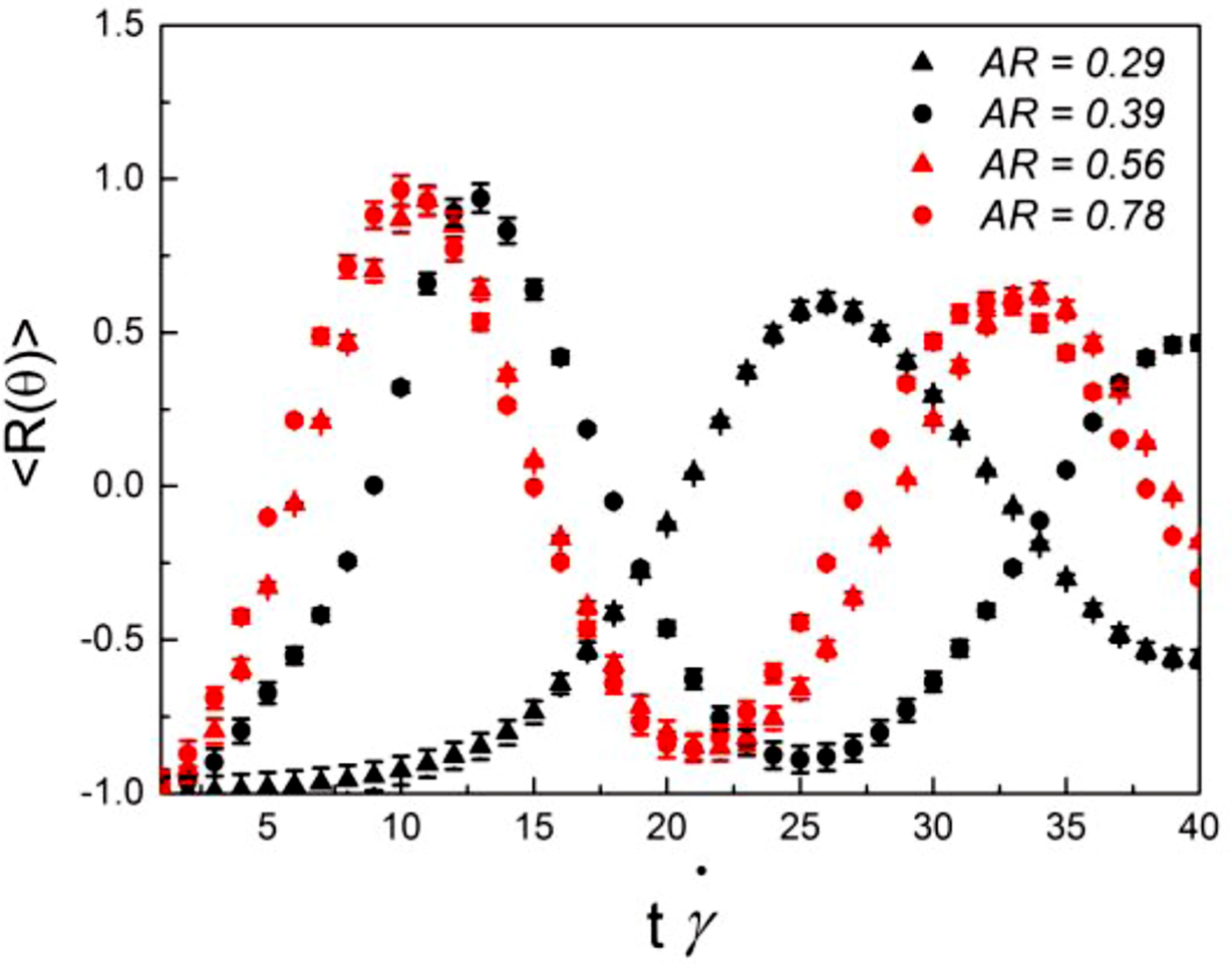
Figure 10 shows the results of determinant of rotation matrix for AR = 0.29–0.78 as a function of time, which was also averaged over particles. The rotation matrix R(θ) in this study is a matrix that corresponds to the linear transformation of a rotation of particle. In R², the matrix, which was considered by a counter clockwise angle θ when rotating (an axis of rotation was the center of particle), has the following form:

The cases for AR = 0.39, 0.56, 0.78 exhibited similar. However, the case AR = 0.29 showed the long wavelength than other cases with increasing t. Furthermore, the elongated particle by the rotational motions increased the particle-particle interactions that can also hinder the rotation as obstacles.

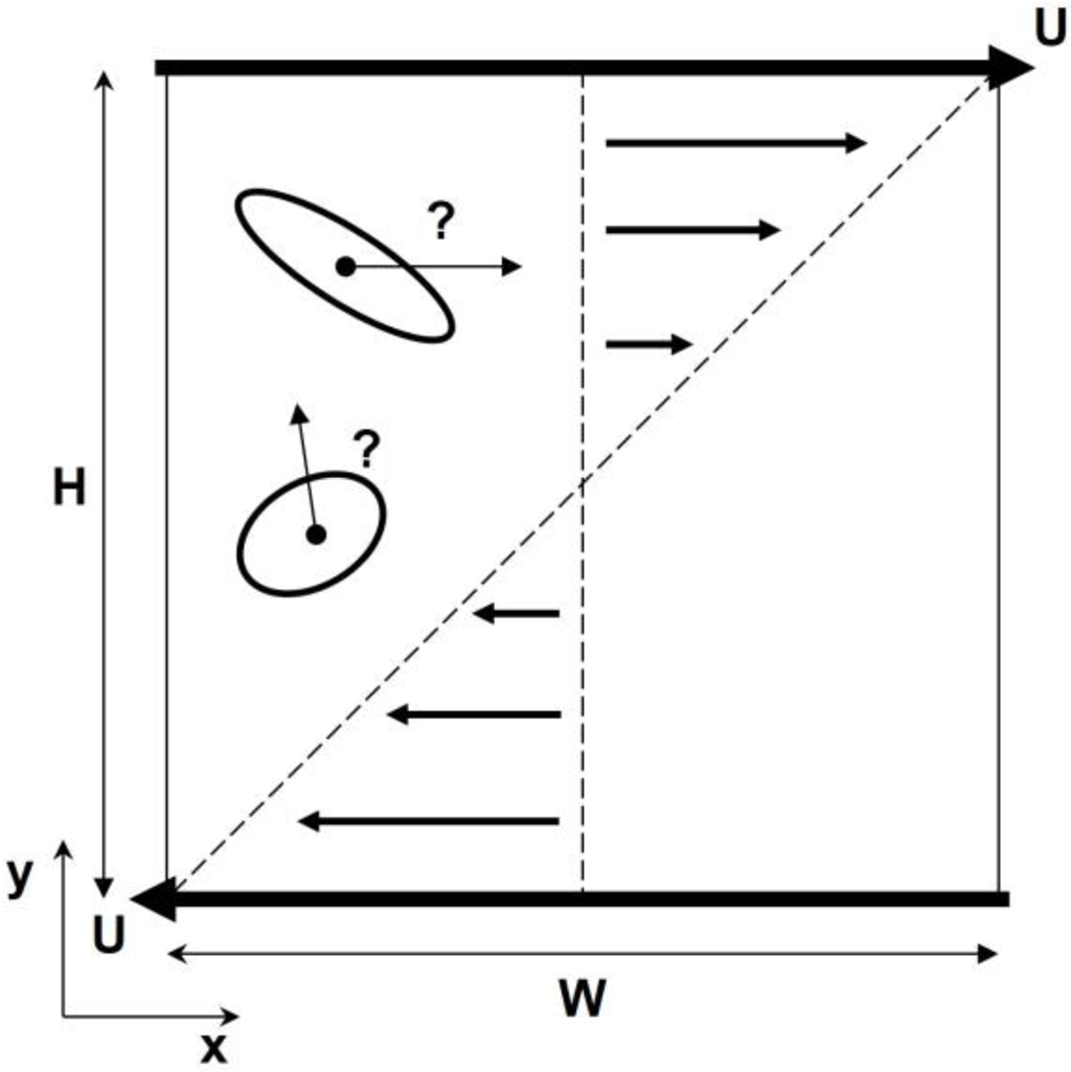
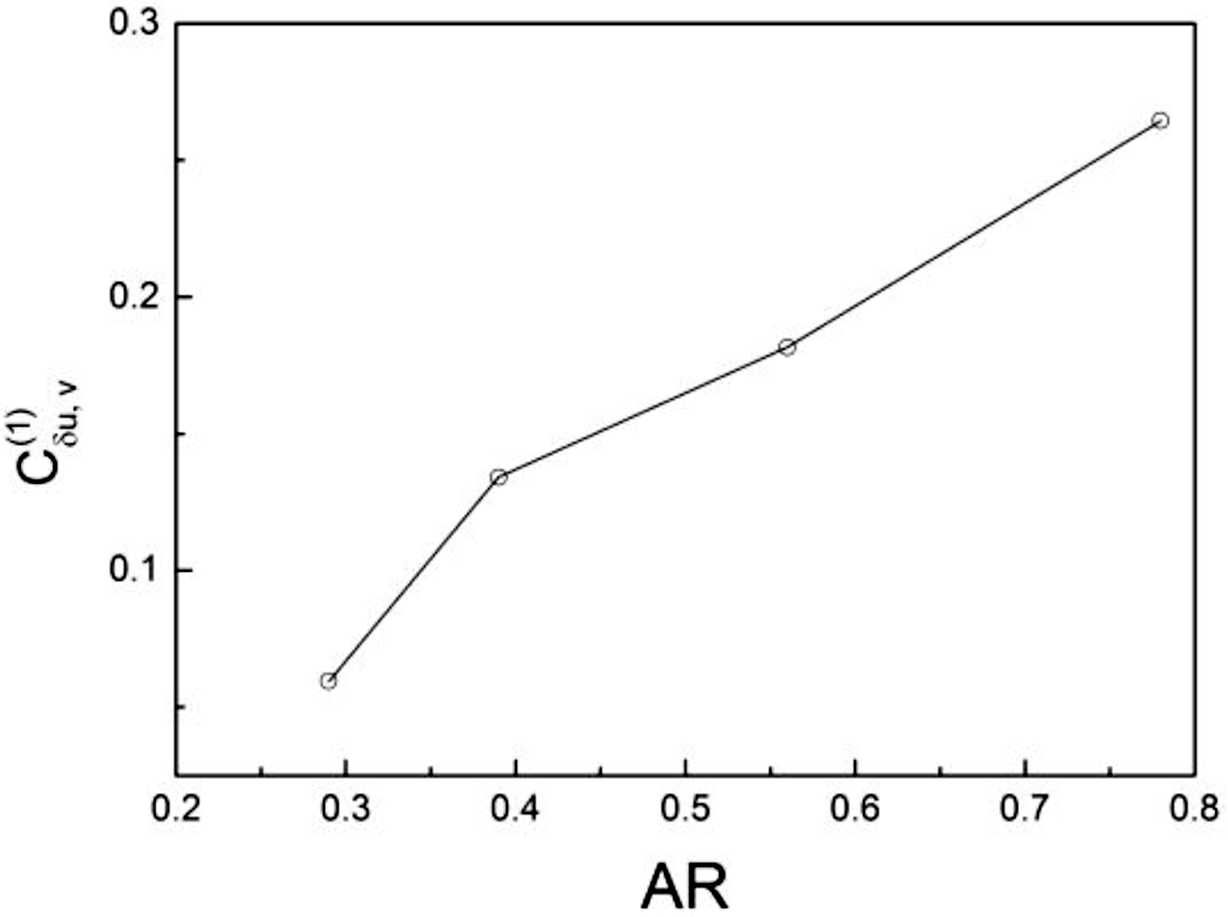
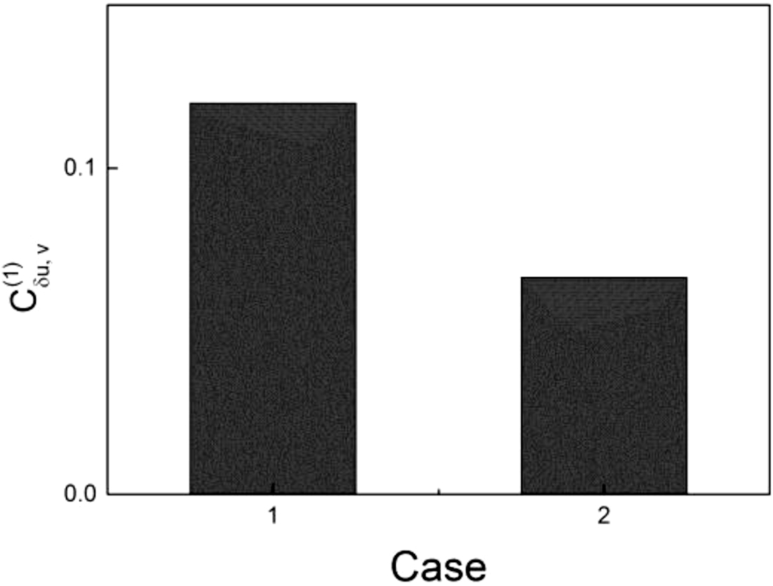
To elucidate the nonlinear dynamics of the particles, we used Lyapunov vectors δu⁽ⁱ⁾(t) indexed by i = 1,2,....³⁸ Each Lyapunov vector, δu⁽ⁱ⁾(t), consisted of translational perturbations, {δr_j⁽ⁱ⁾(t)}, and velocity perturbations, {δv_j⁽ⁱ⁾(t)}, for all particles j. These time-dependent Lyapunov vectors provided information about the heterogeneous dynamics from our calculated results. To evaluate the correlation between the first Lyapunov vectors and the velocity magnitude fields, the cross-correlation was defined as follows:

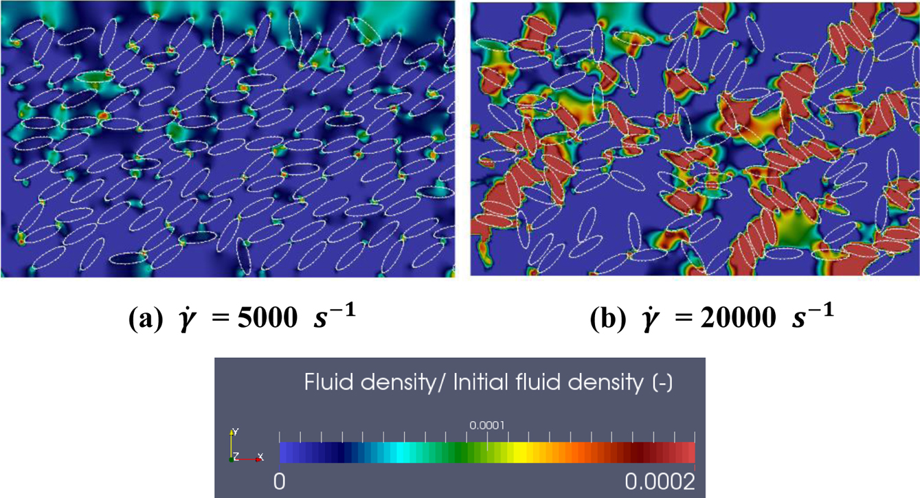
The particle distributions with varying  ( = 5000, 20000 s^-1) are illustrated in Figures 12. For = 5000 s^-1, the particles followed the direction of the flow, and the high-density distribution regime was reduced compared with the previous cases shown in Figure 7(b). However, the over-crowding region was extended for = 20000 s^-1, and particle clusters elongated. Concentrated particle regions due the flow deflection increased the local shear rate and created a disordered state. Some of the particles formed high packing fraction regions. The increased shear force accelerated the concentrated density distribution.

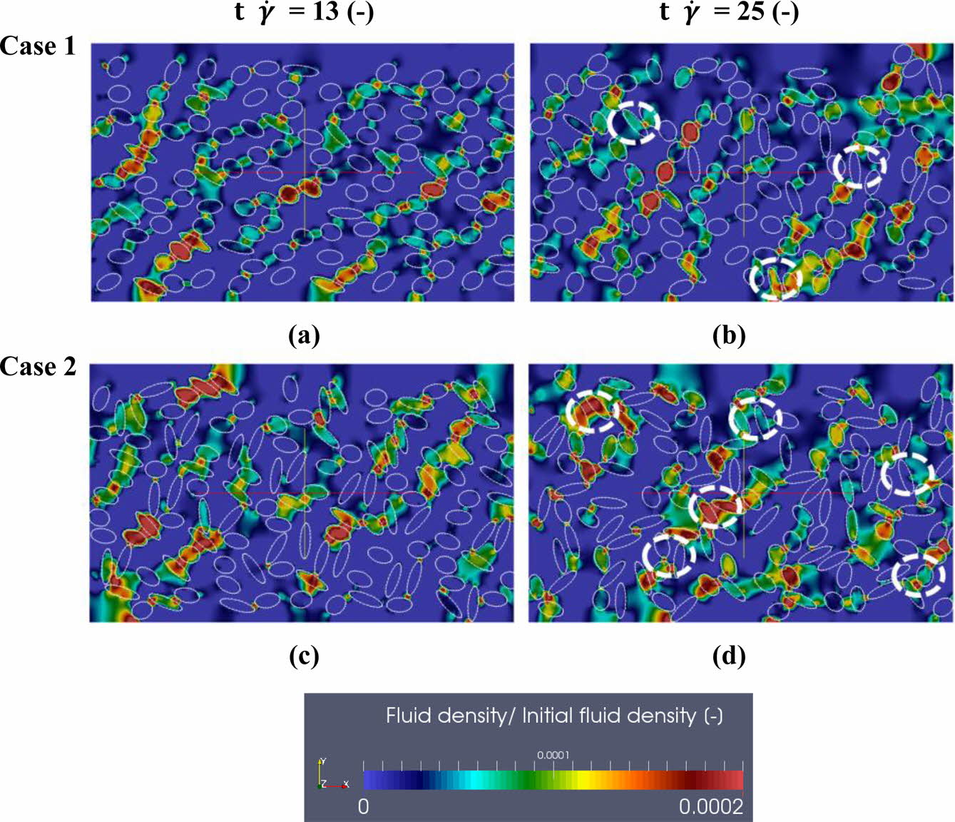
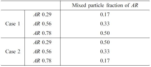
To elucidate the effect of mixed particle shapes in the system, we examined two cases containing mixed three different types of particles (AR = 0.29, 0.56, and 0.78), in which fractions for the different particle types were changed, as summarized in Table 2. As shown in Figures 13, for cases 1 and 2, at t= 13, the particles were uniformly distributed in the suspension. Such behavior resulted from the ordered state of the particles under the applied shear, and the particles aligned themselves to the shear direction. At t  = 25, for cases 1 and 2, net clusters and structures were formed by the elongated particles (illustrated as white dot circles in Figures 13 (b) and (d)). The elongated particles (AR = 0.29) acted as bridges that could act as obstacles and create interconnections between the different types particles (AR = 0.56, 0.78), resulting in strong interactions due to the specific structures of the particles. Such interactions occurred due to the greater number of the surface connections. As the number of elongated particles (AR = 0.29) increased, for case 2, the positions of the jamming clusters partially reinforced the clusters, making it difficult to strip particles. Thus, the cooperation with lower AR particles allowed aggregation to occur more easily than when only nearly spherical particles were present.

Figure 14 shows the cross-correlation calculated using eq. (17) for different mixing fractions of various particles. The values were lower for case 2, in which elongated particles acted as bridges.

LBIBDEM simulations were used to examine aggregates of carbon black ellipsoid particles in shear flow. Each case was classified by the ellipsoid aspect ratio. We observed that the particles for each case exhibited different positions and concentrations due to their shapes by shear. The partially concentrated particle groups consisted of the elongated particles showed that the x-directional velocity was intensive. The rotational motions were crucial for determining particle positions due to the elongated surfaces that could be obstacles. There was a greater amount of particle rearrangement if the particle aggregate shapes were nearly spherical. The elongated particles decreased the amount of rearrangement of partially grouped particles as bridges.

This study to examine the varying shaped particles behavior is important to many engineering systems involving coupled flow, mass transport.